Project Petridish: Efficient forward neural architecture search

Date de publication December 9, 2019

Par Debadeepta Dey , Principal Researcher

Partagez cette page

Having experience in deep learning doesn’t hurt when it comes to the often mysterious, time- and cost-consuming process of hunting down an appropriate neural architecture. But truth be told, no one really knows what works the best on a new dataset and task. Relying on well-known, top-performing networks provides few guarantees in a space where your dataset can look very different from anything those proven networks have encountered before. For example, a network that worked well on satellite images won’t necessarily work well on the selfies and food photos making the rounds on social media. Even when a task dataset is similar to other common datasets and a bit of prior knowledge can be utilized by starting with similar architectures, it’s challenging to find architectures that satisfy not only accuracy, but also memory and latency constraints, among others, at serving time. These challenges could lead to a frustrating amount of trial and error.

In our paper “Efficient Forward Architecture Search,” (opens in new tab) which is being presented at the 33rd Conference on Neural Information Processing Systems (NeurIPS) (opens in new tab), we introduce Petridish, a neural architecture search algorithm that opportunistically adds new layers determined to be beneficial to a parent model, resulting in a gallery of models capable of satisfying a variety of constraints for researchers and engineers to choose from. The team behind the ongoing work is comprised of myself, Carnegie Mellon University PhD graduate Hanzhang Hu (opens in new tab), and John Langford (opens in new tab), Partner Research Manager; Rich Caruana (opens in new tab), Senior Principal Researcher; Shital Shah (opens in new tab), Principal Research Software Engineer; Saurajit Mukherjee (opens in new tab), Principal Engineering Manager; and Eric Horvitz (opens in new tab), Technical Fellow and Director, Microsoft Research AI.

With Petridish, we seek to increase efficiency and speed in finding suitable neural architectures, making the process easier for those in the field, as well as those without expertise interested in machine learning solutions.

Neural architecture search—forward search vs. backward search

The machine learning subfield of neural architecture search (NAS) aims to take the guesswork out of people’s hands and let algorithms search for good architectures. While NAS experienced a resurgence in 2016 (opens in new tab) and has become a very popular topic (see the AutoML Freiburg-Hannover website (opens in new tab) for a continuously updated compilation of published papers), the earliest papers on the topic date back to NeurIPS 1988 (opens in new tab) et NeurIPS 1989 (opens in new tab). Most of the well-known NAS algorithms today, such as Efficient Neural Architecture Search (ENAS) (opens in new tab), Differentiable Architecture Search (DARTS) (opens in new tab), and ProxylessNAS (opens in new tab), are examples of backward search. During backward search, smaller networks are sampled from a supergraph, a large architecture containing multiple subarchitectures. A limitation of backward search algorithms is that human domain knowledge is needed to create a supergraph in the first place. In contrast, Petridish is an example of forward search, a paradigm first introduced 30 years ago by Scott Fahlman and Christian Lebiere of Carnegie Mellon University in that 1989 NAS NeurIPS paper. Forward search requires far less human knowledge when it comes to search space design.

Petridish, which was also inspired by gradient boosting, creates as its search output a gallery of models to choose from, incorporates stop-forward and stop-gradient layers in more efficiently identifying beneficial candidates for building that gallery, and uses asynchronous training.

Figure 1: Petridish, a neural architecture search algorithm that grows a nominal seed model during search by opportunistically adding layers as needed, comprises three phases.

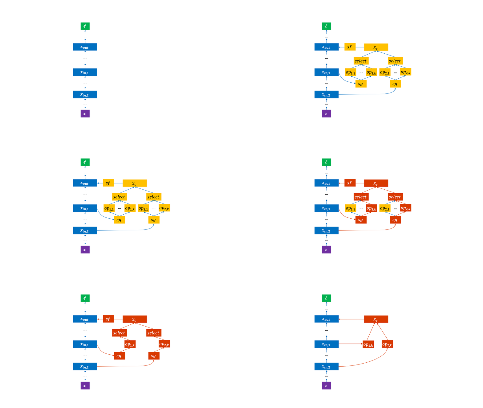
(opens in new tab) Figure 1: Petridish, a neural architecture search algorithm that grows a nominal seed model during search by opportunistically adding layers as needed, comprises three phases. Phase 0 starts with the small parent model. In Phase 1, a large number of candidates is considered for addition to the parent. If a candidate is promising, then it’s added to the parent in Phase 2. Models in Phase 2 that lie near the boundary of the current estimate of the Pareto frontier (see Figure 2) are then added to the pool of parent models in Phase 0 so they have the chance to grow further.

Overview of Petridish

There are three main phases to Petridish:

PHASE 0: We start with some parent model, a very small human-written model with one or two layers or a model already found by domain experts on a dataset.
PHASE 1: We connect the candidate layers to the parent model using stop-gradient et stop-forward layers and partially train it. The candidate layers can be any bag of operations in the search space. For example, for vision tasks, we set the candidates to be 3×3 and 5×5 dilated convolutions, 3×3 and 5×5 separable convolutions, 3×3 max pooling, 3×3 average pooling, and identity. Using stop-gradient and stop-forward layers allows gradients with respect to the candidates to be accumulated without affecting the model’s forward activations and backward gradients. Without the stop-gradient and stop-forward layers, it would be difficult to determine which candidate layers are contributing what to the parent model’s performance and would require separate training if you wanted to see their respective contributions, increasing costs. By leaving the parent model unaffected by the candidate layers, we’re able to independently evaluate each candidate simultaneously.
PHASE 2: If a particular candidate or set of candidates is found to be beneficial to the model, then we remove the stop-gradient and stop-forward layers and the other candidates and train the model to convergence. The training results are added to a scatterplot, naturally creating an estimate of the Pareto frontier. A Pareto frontier encodes the relationship between different objectives of a multi-objective optimization problem where there can’t be gains in one objective without giving up something in the other. Only those models that have a realistic chance of improving the estimate of the Pareto frontier get moved to the parent queue in Phase 0.

Explicitly maintaining a Pareto frontier, like the one represented by Figure 2, allows researchers, engineers, and product groups to more easily determine the architecture that achieves the best combination of properties they’re considering for a particular task. With Figure 2, for example, they can more easily answer questions such as what is the best-performing architecture available given a certain amount of floating-point operations per second (FLOPS) at serving time. This is crucial in production environments, where accuracy, FLOPS, and other metrics like serving latency, memory, and cost are important considerations. Once a search has been completed, if the need for a model meeting different constraints arises, all the team has to do is look it up on the plot without having to redo the architecture hunt.

All three phases are executing concurrently in a distributed manner with each phase maintaining its own queue of models where each queue is cleared by a pool of worker processes in parallel.

Figure 2: Petridish maintains an estimate of the Pareto frontier and makes it easier to see the tradeoff between accuracy, FLOPS, memory, latency, and other criteria. Those models along the Pareto frontier (red line) make up the search output, a gallery of models from which researchers and engineers can choose.

Candidate selection

In Phase 1, for a candidate to be selected for incorporation into the model, we apply L1 regularization to all the candidates and greedily select the candidates that have the highest weight. L1 regularization is commonly used in feature selection to induce sparsity over a set of features so that one can effectively get the most predictive power out of the least number of additional features. Petridish should remind some readers of gradient boosted machines (GBMs), where additional capacity is sequentially added—for example, in a gradient boosted forest—to minimize residual loss.

The construction of Petridish makes it particularly amenable to warm-starting from a previously known model, which is important, as datasets continually change in size and character, a common occurrence in production environments.

Summary of results

On CIFAR-10 (opens in new tab), Petridish achieves 2.75 ±0.21 percent average test error, with 2.51 percent as the best result, using only 3.2M parameters and five GPU days of search time on the popular cell search space. On the more general and bigger macro search space, Petridish achieves 2.85 ±0.12 percent average test error, with 2.83 percent as the best search, using only 2.2M parameters. This is state of the art on a much bigger search space at a similar number of parameters and dispels the common myth that macro search spaces are difficult to deal with and cannot easily achieve competitive performance, opening the door to interesting families of architectures researchers might not have previously considered.

On transferring the models found on CIFAR-10 to ImageNet (opens in new tab), Petridish achieves 28.7 ±0.15 percent top-1 test error, with 28.5 percent as the best result, using only 4.3M parameters on the macro search space. On the cell search space, Petridish achieves 26.3 ±0.20 percent top-1 test error, with 26.0 percent as the best result, using 4.8M parameters. Again, we show that macro search spaces that don’t need a prior human-designed supergraph can be quite competitive, and more research to unlock performance from such expressive spaces is needed.

While we’ve demonstrated Petridish on CIFAR-10/100, ImageNet and also Penn Treebank (opens in new tab), which are commonly accepted NAS datasets, we’re trying it out on a number of diverse datasets in vision and language and invite the community to do the same and report back their experiences. All source code for Petridish is openly available (opens in new tab) (under MIT license) using TensorFlow 1.12. We’re writing a more robust distributed version in PyTorch, which will appear shortly at the same repository.

This work was spearheaded by Hanzhang Hu, a Carnegie Mellon University PhD graduate, during a Microsoft Research summer internship. Team members Debadeepta Dey, John Langford, Rich Caruana, and Eric Horvitz served as advisors on the work.