This is a common story among experimenters: you have a hypothesis to test, you code the change you want to deploy, and you design an A/B test to properly measure the impact of the change on the user. After the A/B test concludes, you don’t observe any statistically significant movements in the metrics. This can occur for one of two reasons: either the change tested doesn’t have an impact on the user, or the change does have an effect but the metrics computed are unable to detect the effect. How can we maximize the chance of detecting an effect when there is one? And how can we increase our confidence that there is no treatment effect when the metrics have no stat-sig movement?

Metric sensitivity analysis helps us quantify how good the metric is at detecting a treatment effect when the change tested in fact has one. The more sensitive a metric, the higher the chance to detect a feature impact, if any. Read the other blog post (opens in new tab) we wrote for high-level overview about why you should care about metric sensitivity and how you can measure it.

Assessing a metric’s sensitivity requires analyzing two aspects of the metric: statistical power (evaluated by the minimum Detectable Treatment Effect (DTE) during power analysis) and movement probability (the probability that a metric will move in a statistically significant manner). Experimenters typically focus on statistical power, but movement probability plays an essential role in the sensitivity of a metric: If a metric is unlikely to move even if the feature or change being tested has a significant impact, the A/B test won’t provide actionable results.

In this blog post, we share:

• How to use statistical power and movement probability to understand metric sensitivity.
• Methods for assessing whether a metric is sensitive enough to detect feature impact – and how we applied them to Microsoft Teams metrics.
• Tips for designing sensitive metrics.

Decomposing Metric Sensitivity

In their analysis of metric actionability, Deng and Shi [1] decompose sensitivity into two components: statistical power and movement probability. Both components play important roles in assessing a feature’s impact successfully.

Assume a feature has an impact on a metric, i.e., the alternative hypothesis is true. Under the alternative hypothesis \( H_1\):

Prob[Detecting the treatment effect on the metric] = \(Prob(H_1)Prob(p<0.05|H_1)\).

\( Prob(p<0.05|H_1)\) is the term for statistical power, the probability of accepting the alternative hypothesis if it is true. It is related to effect size, sample size and significance level. Power analysis allows you to estimate any of these variables, given specific values of the remaining ones (check out this blog post [2] that introduces the basic concepts of statistical power and how to compute it). Experimenters usually evaluate the statistical power by estimating the minimum DTE, which is effect size, given a specific setting of the remaining parameters (i.e., 80% power, 0.05 significance level and a sample size reflecting the typical number of users in an A/B test for that product). \( Prob(H_1)\) is the term for movement probability, representing how often the feature causes the treatment effect under \( H_1\).

Next, we talk about methods for assessing metric sensitivity considering both components.

• Power analysis to verify that the minimum DTE is attainable.
• Movement analysis performed on historical A/B tests:
  1. Movement confusion matrix to study the alignment between the observed metric movement and the expected effect from each historical A/B test.
  2. Observed movement probability to compare the sensitivity of different metrics based on their behavior within the historical A/B tests.

We will illustrate these methods with an example from Microsoft Teams where they evaluated one of their top metrics’ sensitivity – Time in App. The metric, which measures high-level user engagement with the product, is an indicator that the app is delivering value to the users.

Power Analysis

With the results of power analysis, the metric authors can discuss with the feature team whether the minimum DTE for the metric is attainable in typical A/B tests. If the value is in percentage, it is good to convert it to absolute value to get a sense of the magnitude of the required change. If the minimum DTE is far beyond what is expected in a typical A/B test, the metric may rarely move. In the case of Microsoft Teams, Time in App has 0.3% as minimum DTE with full traffic in 1 week. The team mapped the percentage to an absolute increase in the metric, and they were satisfied with the statistical power: they expect that feature changes would reasonably lead to such an increase in Time in App and hence the minimum DTE was achievable.

Movement analysis

To evaluate a metric’s sensitivity, the metric authors should study the metric behavior on historical A/B tests results. Historical A/B tests are a great tool for evaluating metrics – they are referred to as “Experiment Corpus” in [3] and are heavily used to assess the quality of a proposed metric. The greater the quantity of historical A/B tests available, the more actionable the study results would be.

The study uses two common types of corpus. Labeled corpus consists of tests where there is high confidence that a treatment effect exists. That confidence is built by examining many metric movements to check if they align with the hypothesis of the test, deep dives and offline analyses that add more evidence to the correctness of the hypotheses of the A/B tests. Unlabeled corpus consists of randomly selected tests and helps evaluate the overall movement probability.

1. Movement Confusion Matrix

The confusion matrix below helps understand if the metric moves as expected. The expectation is indicated by the label in the matrix below and is supported by analyzing metrics and deep diving on the A/B test. In the table, the left column covers A/B tests where the alternative hypothesis \( H_1\) is true and the right one covers those where \( H_0\) is true. Each test from the labeled corpus can fit into one of the two columns.

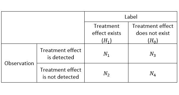
To fill the matrix, compute the metric on all the A/B tests in the labeled corpus. A treatment effect is detected when the metric has a statistically significant movement. Otherwise, a treatment effect is not detected.

Once you have the metric movements, check tests covered by \( N_1\) to see if the metric has the same direction as expected. For tests where metric movements are in the opposite direction, metric authors should investigate further. Is that because the previous labeling analysis was insufficient and the expected direction is incorrect? Or is that because the metric diverges from the real movement in some cases? In the first case, update the label of the A/B test. Otherwise, the metric can be untrustworthy and can lead to incorrect decision making. Metric authors should consider using an alternative metric that better aligns with the product.

The confusion matrix summarizes the behavior of the metric on the labeled corpus. A metric that is sensitive will have a large \( \frac{N_1}{N_1+N_2}\), as close to 1 as possible. A robust metric (i.e., one that is less susceptible to noisy movements) will have \( \frac{N_3}{N_3+N_4}\) that is very close to the significance level or false positive rate.

Microsoft Teams expected Time in App to move when treatment effect existed in supporting metrics such as chat or call actions. They found several tests with promising impact, but Time in App missed catching those, with \( \frac{N_1}{N_1+N_2}\) close to 0.

2. Observed Movement Probability

While a labeled corpus can be very useful for metric evaluations, it takes a lot of time and effort to label the A/B tests in a confident manner. An unlabeled corpus can be used to compare sensitivity among various candidate metrics, as Deng and Shi described In [1]. To do the comparison, we first compute the observed movement probability for each candidate metric: this is the proportion of A/B tests where the metric’s movement was statistically significant (p-value < 0.05). To compute this probability using the unlabeled corpus, the metric authors can generate a confusion matrix for each candidate similar to the one above, with the two columns collapsed into one. This corresponds to \( \frac{N_1+N_3}{N_1+N_2+N_3+N_4}\). Note that labels for the A/B tests are not needed here since we are only studying the movement of one metric compared to others.

To properly compare the movement probability among metrics, we first decompose it by the correctness of the alternative hypothesis. The observed movement probability can be written as:

\( Prob(H_1)Prob(p<0.05|H_1) + Prob(H_0)Prob(p<0.05|H_0)\).

The first term represents the probability that a real treatment effect exists and is successfully detected. The second term is the bias introduced by the metric’s false positive movement in the A/B tests with no treatment effect. The bias term is bounded at 5%, the significance level we use in our analysis.

This makes the observed movement probability a biased estimation of the real movement probability of each metric, with the bias upperbounded by 5%. Hence, the observed movement probability can still be used to compare sensitivity between metrics as long as the difference between the observed probabilities is larger than 5% – the upper bound of bias.

Microsoft Teams collected dozens of historical A/B tests, and the observed movement probability for the Time In App metric was much lower than that of several other metrics in use. This indicated that Time in App has much lower sensitivity and the metric authors need to improve it before it can be properly used in A/B tests.

Tips for designing sensitive metrics

So, you performed the analysis above and you found your metric to be insensitive. Before you trash the metric and start from scratch, below are some tips and tricks to help metric authors improve the sensitivity of some metrics: variations on metric definitions help improve the overall sensitivity, and variance reduction technique efficiently improves statistical power.

Metric design

Sometimes a metric is determined to be insensitive yet it still accurately measures what the team wants to assess in an A/B test. Applying techniques from A/B metric design [4,5] is one of the simplest ways to increase its sensitivity. Below are some techniques that can help you increase the sensitivity of your metric.

Apply a transformation to the metric value

One straightforward way of improving the sensitivity of a metric is reducing the impact of outliers. The transformations below change the computation of the metric to minimize the impact or remove it all together.

• • Capping the value of the metric at a fixed maximum value can greatly reduce the impact of outliers which usually hurt sensitivity.
  • Apply the Log function on the metric value: \( x \rightarrow log(1+x)\). This transformation gives less weight to extreme large values when the distribution is skewed, which helps detect smaller metric movement.
  • Change of metric’s aggregation level impacts the weight assigned to each unit. See [6] about how single-average and double-average differ in tenant randomized tests.

Use alternative metric types

Typically, A/B metrics are averaged across the randomization units. These are Average metrics and Time in App per User is one such example. However, using alternative methods to aggregate the metric can help increase its sensitivity. Below are some other metric types we can use:

• • Proportion metrics measure the proportion of the units satisfying a condition, e.g., % Users with Time in Channel. A proportion metric is easier to move, compared to the other types.
  • Conditional average metric is similar to average metric, except that the unit base is under a condition, e.g., Time in App per Active User. The statistical power will be improved if the numerator and denominator are correlated.
  • Percentile metric is usually used to monitor the extreme case, such as 99 Percentile of Time in App.

Try proxy metrics

If a metric represents a long-term goal, such as overall user satisfaction, it might be hard to move in the short period of an A/B test. Consider finding proxy metrics by predictive models [7].

Variance Reduction

CUPED (Controlled-experiment Using Pre-Experiment Data) [8] is one Variance Reduction method, leveraging the data prior to the A/B test to remove explainable variance during the test. It has been shown to be effective and is widely used in A/B tests at Microsoft.

Microsoft Teams tried several types of metric design and Variance Reduction for Time in App. Following the steps for assessing sensitivity, they finally chose Log of Capped Time in App as the alternative to Time in App, with Variance Reduction applied whenever possible during A/B test results analysis.

Summary

Experimenters need sensitive metrics to detect a feature impact. But sensitivity can’t be determined by statistical power alone. Metric authors could design alternative metrics and then select the best based on the evaluation methods mentioned above. Consider how each metric fulfills the following qualities. If no metric fulfills all of them, choose the one that meets most of them.

• Feature teams agree that the minimum DTE of the metric can be achieved.
• In the confusion matrix, the movement direction is always explainable for A/B tests covered by \( N_1\).
• The metric has high \( \frac{N_1}{N_1+N_2}\) in the confusion matrix and \( \frac{N_3}{N_3+N_4}\) close to the significance level.
• The metric should have large observed movement probability compared with other candidates.

We hope this article helps metric authors explore additional approaches for assessing and fine-tuning metric sensitivity.

 

– Wen Qin and Widad Machmouchi, Microsoft Experimentation Platform

– Alexandre Matos Martins, Microsoft Teams

References

[1] A. Deng and X. Shi, “Data-Driven Metric Development for Online Controlled Experiments: Seven Lessons Learned,” in Proceedings of the 22nd ACM SIGKDD International Conference on Knowledge Discovery and Data Mining – KDD ’16, San Francisco, California, USA, 2016, pp. 77–86, doi: 10.1145/2939672.2939700.

[2] B. Jason, “A Gentle Introduction to Statistical Power and Power Analysis in Python.” https://machinelearningmastery.com/statistical-power-and-power-analysis-in-python/.

[3] P. Dmitriev and X. Wu, “Measuring Metrics,” in Proceedings of the 25th ACM International on Conference on Information and Knowledge Management – CIKM ’16, Indianapolis, Indiana, USA, 2016, pp. 429–437, doi: 10.1145/2983323.2983356.

[4] W. Machmouchi and G. Buscher, “Principles for the Design of Online A/B Metrics,” in Proceedings of the 39th International ACM SIGIR conference on Research and Development in Information Retrieval, Pisa Italy, Jul. 2016, pp. 589–590, doi: 10.1145/2911451.2926731.

[5] R. Kohavi, D. Tang, and Y. Xu, Trustworthy Online Controlled Experiments: A Practical Guide to A/B Testing. Cambridge University Press, 2020.

[6] J. Li et al., “Why Tenant-Randomized A/B Test is Challenging and Tenant-Pairing May Not Work.” https://www.microsoft.com/en-us/research/group/experimentation-platform-exp/articles/why-tenant-randomized-a-b-test-is-challenging-and-tenant-pairing-may-not-work/.

[7] S. Gupta, R. Kohavi, D. Tang, and Y. Xu, “Top Challenges from the first Practical Online Controlled Experiments Summit,” ACM SIGKDD Explor. Newsl., vol. 21, no. 1, pp. 20–35, May 2019, doi: 10.1145/3331651.3331655.

[8] A. Deng, Y. Xu, R. Kohavi, and T. Walker, “Improving the sensitivity of online controlled experiments by utilizing pre-experiment data,” in Proceedings of the sixth ACM international conference on Web search and data mining – WSDM ’13, Rome, Italy, 2013, p. 123, doi: 10.1145/2433396.2433413.

 

Opens in a new tab